Chinchilla review
Whenever I see a discussion online about the current generation of LLMs, there is an inherent assumption and extrapolation that these technologies will keep improving with time. Why do we think that? The approximate answer is because of scaling laws which suggest indefinite improvement for the current style of transformers with additional pre-training data and parameters. This blog post delves into the intricacies of these scaling laws and examines how they guide the development of more powerful and efficient LLMs. I will be as comprehensive as I can (with the math knowledge I have) including parts about the scaling law origins, recent finding and their implications.
First we will try to understand the basic variables involved in scaling large language models:
- Parameters of the model. We will be using it as a proxy for size and its a broad term that includes both the weights and biases of a model. The size of a neural network typically refers to the number of trainable parameters it contains.
- Weights and biases are the values learned during the training process and they represent the “weight” of a connection between neurons of different layers.
- Parameters and hyper parameters are different. Hyper parameters are your model config settings like learning rate, no. of epochs, batch size etc and aren’t learned from the data itself. They are set during time of training and are irrelevant to our discussion
- Compute. Usually represented in FLOPS(basically no. of arithmetic operations per second). Here, we use it to estimate training complexity of the neural net. While calculating FLOPs to dollars is not straightforward and will depend on hardware used and energy costs, we will use it as a proxy for money spent.
- Tokens. This is just a proxy for the size of the training dataset
- Performance. This is nothing but how the trained model performs on certain benchmarks designed to evaluate across axis like classification accuracy, generalization ability, efficiency and task specific metrics.
- Compute Optimal. Its basically a concept which determines how to extract the most performance out of your model given a constrained compute budget and model size.
There were three seminal publications in this field as listed below. This post will focus mainly on the Chinchilla paper
- Kaplan Paper
- Chinchilla update to scaling laws (Mistral AI co-founder was one of the first authors)
- OpenAI scaling laws (Kaplan is a co-founder at Anthropic)
The first Kaplan paper basically showed that there is a power law relationship between the number of parameters in a LLM and its performance. Kaplan paper suggests that to train larger models, increasing the number of parameters is 3x more important than increasing the size of the training set This implication basically led to larger and larger models getting trained expecting performance improvements. While the following Chinchilla paper comes to a similar conclusion, they estimate that large models should be trained for many more training tokens than recommended by the Kaplan paper. Training an optimal model requires about 20x more tokens than parameters.
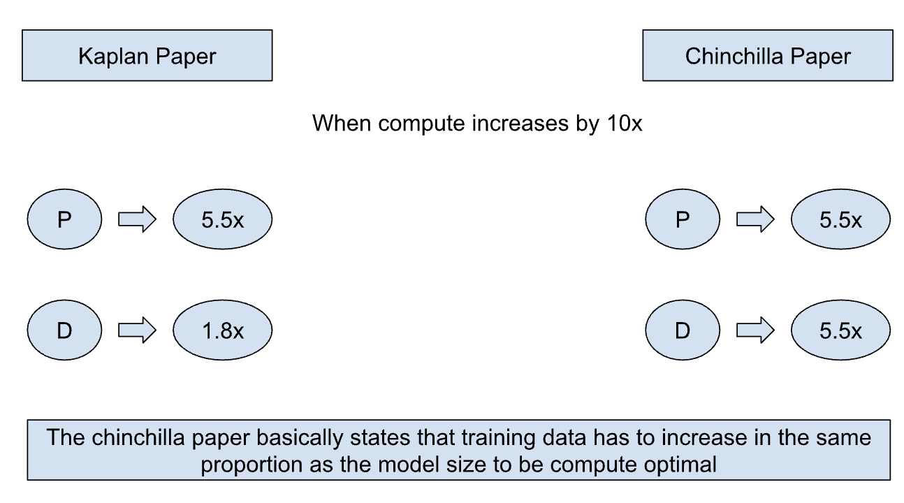
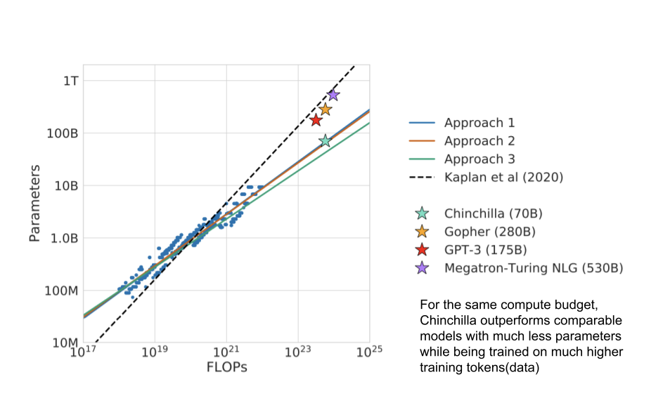
So in around late 2021, the Deepmind team went on to train about 400 models ranging from 70 million to 16 billion parameters on datasets ranging from 5 to 500 billion tokens. They did a bunch of experiments and found some interesting results. Specifically, given a 10× increase computational budget, Kaplan paper suggested that the size of the model should increase 5.5× while the number of training tokens should only increase 1.8×. Instead, Chinchilla states that model size and the number of training tokens should be scaled in equal proportions. To demonstrate this they trained a model (Chinchilla) which had better performance than comparative models for the same compute budget.
How did they find this?
The fundamental question they were trying to answer was “Given a fixed FLOPs budget, how should one trade-off model size and the number of training tokens?” . Its basically an optimization problem where you fix one variable (FLOPs) and try to find the optimal values for parameters and tokens. However, every time they have to test a value for parameters/tokens they have to train a model which costs millions of dollars. For the paper, they trained over 400 models with varying values of parameters and tokens taking certain approaches. Lets look at them below:
- Approach 1: Fix the parameter variable and vary the size of the training tokens
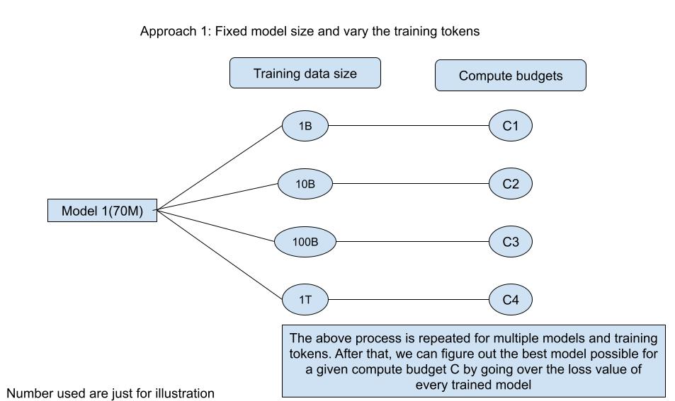
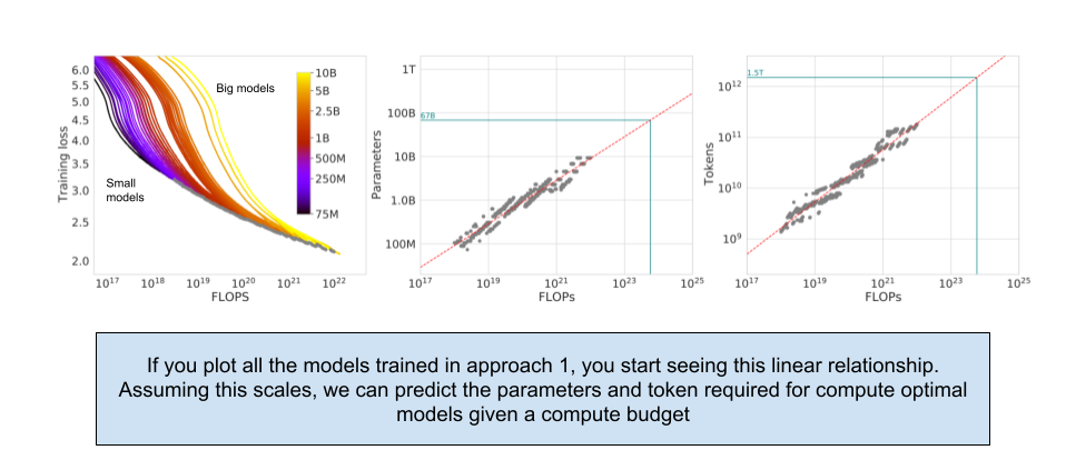
Here, they took a couple models with parameters ranging from 70M to 10B and trained them each on four types of datasets (differentiated by size). Based on this training, they were able to estimate the model with minimum loss (we will use loss as proxy for model performance as far as this blog post is concerned) for a given compute budget. As you see above, they were able to determine the best model (parameters/token) for a given compute budget by looking at the loss value of every trained model.
- Approach 2: Fix the compute budget and vary the number of parameters of the neural network
In the first approach, they fixed the number of parameters of the model and trained them on multiple token sizes. Based on the compute used for each model, they were able to select the model with the ideal parameter/token size for a given budget. In this approach, they fix the amount of FLOPs for each model and vary the number of parameters for each model. According to this approach, Google would have had to train PaLM with about 14 trillion tokens to obtain the optimal loss for a 540B parameters model.
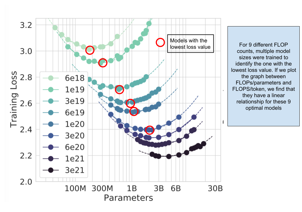
- Approach 3: Take data from first two approaches and try to find a function for loss values
This approach was slightly mathematical in nature and I shall skip directly to the results. We find the model with the lowest loss value for a given compute budget and model size.
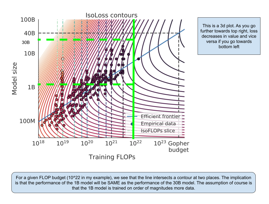
Throughout the three approaches, the paper keeps referencing the Gopher model (which was earlier trained by Deepmind only) to try to demonstrate the optimal values for parameters and tokens given the compute size that was historically used. They find that the optimal model size given the Gopher budget to be a 67B model instead of the 280B they actually trained.
Conclusions
Modern large language models have been oversized unnecessarily. With no added performance, companies have been training massive models wasting resources. Here is a table showing optimal training FLOPs and training token for different model sizes.
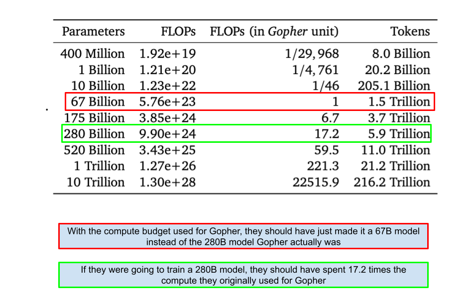
After training more than 400models to prove the above relationships, they train the Chinchilla model to drive the point across. The idea of this model was to take the above relationships and REDO Gopher. They used the same amount of computer budget as Gopher but used 70B parameters and 1.4T tokens to train Chinchilla and it ends up outperforming Gopher is a lot of benchmarks. For the same amount of money spent, they got a better model out basically. Moreover, its cheaper to run inference on smaller models leading to more cost savings over the long run.
Current models are extremely oversized for their performance. Going after parameters is inefficient. While AI labs have been going after larger and larger models, post Chinchilla era dictates that they should be going after massive training data as well. This requires research into more optimization steps and increases in batch sizes (which however has adverse impact on model performance after a point). The problem of maintaining training efficiency while increasing data size becomes very important to solve. We also might be running out of data as this Lesswrong article implies.
Emergent properties
I originally started writing this document to explain the Chinchilla results and ponder over certain emergent behavior to make an educated guess about AGI timelines. An amazing property of LLMs is the emergence of new capabilities as the size of the network increases. In other words, LLMs unpredictably learn to perform new tasks, without having been specifically trained to do so. The system becomes more complex than the sum of the parts. Here is a GIF from the Google PaLM paper showing the same.

We currently don’t know at scale emergent behavior shows up and we can’t even estimate the level of ability or even the potential categories of such abilities. This paper from Google shows that emergent abilities cannot be predicted simply by extrapolating the performance of smaller models. The existence of such emergence also raises the question of whether additional scaling could potentially further expand the range of capabilities of language models or not. On one side, we have the Chinchilla paper showing us that the model performance keeps getting better with increasing parameter and token size. On another side, we have established that emergent behaviors keep popping up with increasing model scale. Ilya Sutskever uses the above to basically explain why next-token prediction is enough for AGI?. Maybe figuring out a relationship between next word prediction accuracy and reasoning abilities could be the way to make current gen LLMs truly intelligent.
The convergence of scaling laws and emergent abilities not only makes me excited for the future of AI but also brings in a new era where the unforeseen capabilities of AGI could revolutionize our understanding of intelligence itself.